Intro to R & R Studio

Author

James Van Slyke

R is the base program for R Studio, it does all the calculations, while R studio is the addition of several windows around R that helps with your analysis

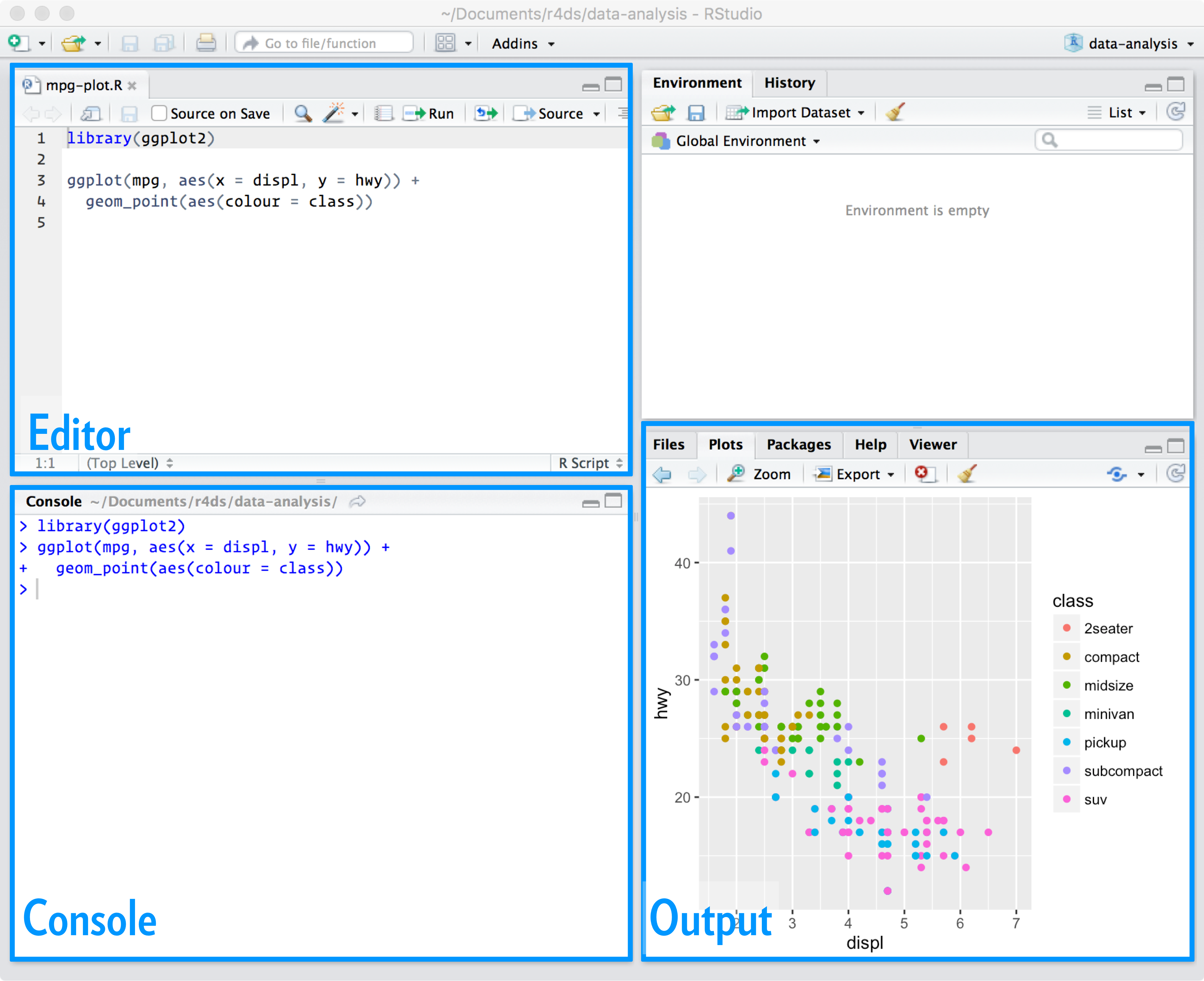
In R Studio, “R” performs calculations in the console. The console is in the lower left window. You can think of the console as a big calculator. You can do all the basics with R.

The Editor is where you write the code and notes to yourself in scripts. The console is where you code gets entered and run and the output is in the lower right hand corner. The upper left hand window is the environment and keeps track of the data and other things used in your analysis.

Here is a picture of what the program looks like and the different sections.

Basic Calculations using R

Addition

x <- 3 + 2
x

[1] 5

Subtraction

x <-  3 - 2
x

[1] 1

Multiplication

x <-  3 * 2
x

[1] 6

Division

x <-  3 / 2
x

[1] 1.5

Exponent

x <- 3^2
x

[1] 9

You’ll notice that the calculations are being saved as what’s called an object. An object is anything you save in R that is related to data or output of a calculation. You can save calculations, databases, words or lots of other stuff.

If you look in the upper right window, under the environment tab, you should notice an x there based on your last calculation. The environment tab saves all the saved objects you are working with in R.

Here’s a couple of examples of objects for you to try

Word <- "Word"
Number <- 1
Calculation <- 3+2

Notice that when you call up a calculation it gives you the answer, not the formula

You can create a sequence of numbers

seq(1,10)

 [1]  1  2  3  4  5  6  7  8  9 10

You can repeat numbers

rep(10, times = 25)

 [1] 10 10 10 10 10 10 10 10 10 10 10 10 10 10 10 10 10 10 10 10 10 10 10 10 10

And of course you can always store it in an object

Repeat <- rep(10, times = 25)
Repeat

 [1] 10 10 10 10 10 10 10 10 10 10 10 10 10 10 10 10 10 10 10 10 10 10 10 10 10

Then you can use that to make a new database

First we’ll add a sequence of numbers to match our repeat variable

Sequence <- seq(1,25)
Sequence

 [1]  1  2  3  4  5  6  7  8  9 10 11 12 13 14 15 16 17 18 19 20 21 22 23 24 25

Then create a dataset using the data.frame command and include the two objects that were just recently created.

Dataset <- data.frame(Repeat, Sequence)
Dataset

   Repeat Sequence
1      10        1
2      10        2
3      10        3
4      10        4
5      10        5
6      10        6
7      10        7
8      10        8
9      10        9
10     10       10
11     10       11
12     10       12
13     10       13
14     10       14
15     10       15
16     10       16
17     10       17
18     10       18
19     10       19
20     10       20
21     10       21
22     10       22
23     10       23
24     10       24
25     10       25

Inspecting data

There’s lots of things you can do with a dataset

Let’s start with one that is already in the R environment iris

It’s a longer dataset, so we’ll start with the head command that just shows the first couple of rows

The top rows and columns of the dataset

head(iris)

  Sepal.Length Sepal.Width Petal.Length Petal.Width Species
1          5.1         3.5          1.4         0.2  setosa
2          4.9         3.0          1.4         0.2  setosa
3          4.7         3.2          1.3         0.2  setosa
4          4.6         3.1          1.5         0.2  setosa
5          5.0         3.6          1.4         0.2  setosa
6          5.4         3.9          1.7         0.4  setosa

We can look at the types of data we have using the str command

str(iris)

'data.frame':   150 obs. of  5 variables:
 $ Sepal.Length: num  5.1 4.9 4.7 4.6 5 5.4 4.6 5 4.4 4.9 ...
 $ Sepal.Width : num  3.5 3 3.2 3.1 3.6 3.9 3.4 3.4 2.9 3.1 ...
 $ Petal.Length: num  1.4 1.4 1.3 1.5 1.4 1.7 1.4 1.5 1.4 1.5 ...
 $ Petal.Width : num  0.2 0.2 0.2 0.2 0.2 0.4 0.3 0.2 0.2 0.1 ...
 $ Species     : Factor w/ 3 levels "setosa","versicolor",..: 1 1 1 1 1 1 1 1 1 1 ...

Notice we have 2 data types, numbers and what are called “factors”

Factors are typically categories of something. In this case, types of iris flowers.

We can check on the names of each of our variables

names(iris)

[1] "Sepal.Length" "Sepal.Width"  "Petal.Length" "Petal.Width"  "Species"

We can look at the row names

rownames(iris)

  [1] "1"   "2"   "3"   "4"   "5"   "6"   "7"   "8"   "9"   "10"  "11"  "12" 
 [13] "13"  "14"  "15"  "16"  "17"  "18"  "19"  "20"  "21"  "22"  "23"  "24" 
 [25] "25"  "26"  "27"  "28"  "29"  "30"  "31"  "32"  "33"  "34"  "35"  "36" 
 [37] "37"  "38"  "39"  "40"  "41"  "42"  "43"  "44"  "45"  "46"  "47"  "48" 
 [49] "49"  "50"  "51"  "52"  "53"  "54"  "55"  "56"  "57"  "58"  "59"  "60" 
 [61] "61"  "62"  "63"  "64"  "65"  "66"  "67"  "68"  "69"  "70"  "71"  "72" 
 [73] "73"  "74"  "75"  "76"  "77"  "78"  "79"  "80"  "81"  "82"  "83"  "84" 
 [85] "85"  "86"  "87"  "88"  "89"  "90"  "91"  "92"  "93"  "94"  "95"  "96" 
 [97] "97"  "98"  "99"  "100" "101" "102" "103" "104" "105" "106" "107" "108"
[109] "109" "110" "111" "112" "113" "114" "115" "116" "117" "118" "119" "120"
[121] "121" "122" "123" "124" "125" "126" "127" "128" "129" "130" "131" "132"
[133] "133" "134" "135" "136" "137" "138" "139" "140" "141" "142" "143" "144"
[145] "145" "146" "147" "148" "149" "150"

We can create a table of a particular variable

We specify the variable we want by using the $ sign

table(iris$Species)


    setosa versicolor  virginica 
        50         50         50

Notice that it automatically makes a table of the counts of each iris type

Anytime we want to look at a specific variable from a dataset, we use the $ sign. Notice when you type in the dataset name followed by the $ you’ll see a little pop-up with all the variables. Just scroll through and select the one you want.

iris$Sepal.Width

  [1] 3.5 3.0 3.2 3.1 3.6 3.9 3.4 3.4 2.9 3.1 3.7 3.4 3.0 3.0 4.0 4.4 3.9 3.5
 [19] 3.8 3.8 3.4 3.7 3.6 3.3 3.4 3.0 3.4 3.5 3.4 3.2 3.1 3.4 4.1 4.2 3.1 3.2
 [37] 3.5 3.6 3.0 3.4 3.5 2.3 3.2 3.5 3.8 3.0 3.8 3.2 3.7 3.3 3.2 3.2 3.1 2.3
 [55] 2.8 2.8 3.3 2.4 2.9 2.7 2.0 3.0 2.2 2.9 2.9 3.1 3.0 2.7 2.2 2.5 3.2 2.8
 [73] 2.5 2.8 2.9 3.0 2.8 3.0 2.9 2.6 2.4 2.4 2.7 2.7 3.0 3.4 3.1 2.3 3.0 2.5
 [91] 2.6 3.0 2.6 2.3 2.7 3.0 2.9 2.9 2.5 2.8 3.3 2.7 3.0 2.9 3.0 3.0 2.5 2.9
[109] 2.5 3.6 3.2 2.7 3.0 2.5 2.8 3.2 3.0 3.8 2.6 2.2 3.2 2.8 2.8 2.7 3.3 3.2
[127] 2.8 3.0 2.8 3.0 2.8 3.8 2.8 2.8 2.6 3.0 3.4 3.1 3.0 3.1 3.1 3.1 2.7 3.2
[145] 3.3 3.0 2.5 3.0 3.4 3.0

Dataframes

Many times we work with datasets using dataframes, which creates an object very similar to a spreadsheet. Notice that when we create a dataframe and add variables to it, the letter c is used before the parentheses, which basically tells R that what follows should be added to the object/variable before it.

Here is a sample dataset

Dataframe <- data.frame(Words = c("One", "Two", "Three", "Four"),
                        Numbers = c(1,2,3,4))

Inspect It

Dataframe

  Words Numbers
1   One       1
2   Two       2
3 Three       3
4  Four       4

You can also view it as a spreadsheet

View(Dataframe)

There’s actually lots of ways to make datasets and we can always import data, which we will learn later.

Different class types in r

Numeric means number

Integer means a number that is not a fraction

check it out

is.numeric(4.2)

[1] TRUE

is.integer(4.2)

[1] FALSE

Characters are strings or words

check it out

is.character("Word")

[1] TRUE

is.character(4)

[1] FALSE

Factors are categories as I described earlier, it can be ordered (like an ordinal scale) or non-ordered

str(iris)

'data.frame':   150 obs. of  5 variables:
 $ Sepal.Length: num  5.1 4.9 4.7 4.6 5 5.4 4.6 5 4.4 4.9 ...
 $ Sepal.Width : num  3.5 3 3.2 3.1 3.6 3.9 3.4 3.4 2.9 3.1 ...
 $ Petal.Length: num  1.4 1.4 1.3 1.5 1.4 1.7 1.4 1.5 1.4 1.5 ...
 $ Petal.Width : num  0.2 0.2 0.2 0.2 0.2 0.4 0.3 0.2 0.2 0.1 ...
 $ Species     : Factor w/ 3 levels "setosa","versicolor",..: 1 1 1 1 1 1 1 1 1 1 ...

The basic structure of R commands

Their are four main elements of every R code

objects
functions
arguments
operators

Basic Structure

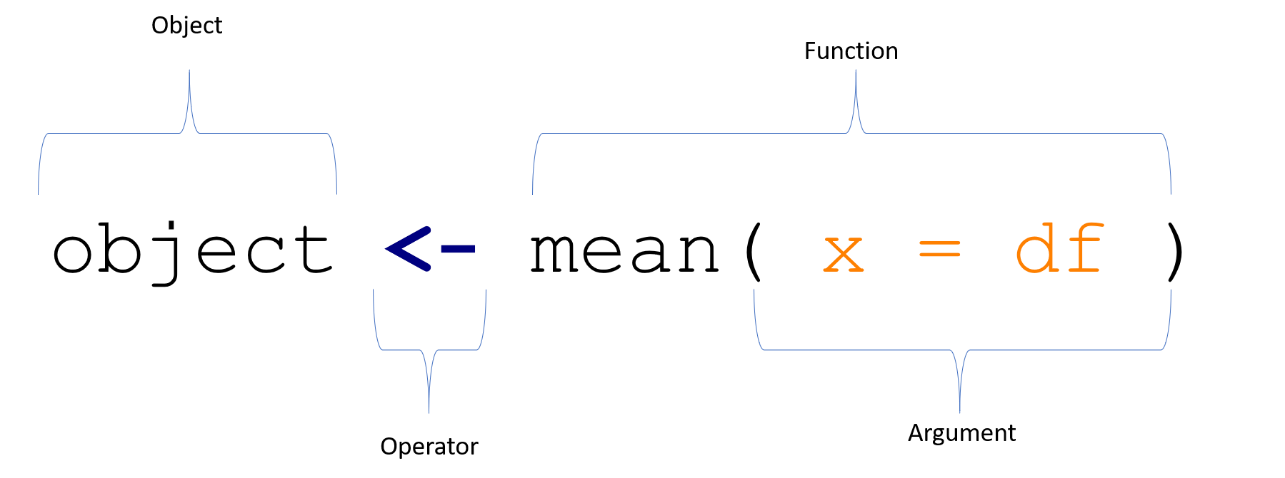
The function mean generates the arithmetic mean of some object

mean(iris$Sepal.Length)

[1] 5.843333

Or we can find the standard deviation

sd(iris$Sepal.Length)

[1] 0.8280661

We can also get a summary of the variable or the dataset as a whole

summary(iris$Sepal.Length)

   Min. 1st Qu.  Median    Mean 3rd Qu.    Max. 
  4.300   5.100   5.800   5.843   6.400   7.900

summary(iris)

  Sepal.Length    Sepal.Width     Petal.Length    Petal.Width   
 Min.   :4.300   Min.   :2.000   Min.   :1.000   Min.   :0.100  
 1st Qu.:5.100   1st Qu.:2.800   1st Qu.:1.600   1st Qu.:0.300  
 Median :5.800   Median :3.000   Median :4.350   Median :1.300  
 Mean   :5.843   Mean   :3.057   Mean   :3.758   Mean   :1.199  
 3rd Qu.:6.400   3rd Qu.:3.300   3rd Qu.:5.100   3rd Qu.:1.800  
 Max.   :7.900   Max.   :4.400   Max.   :6.900   Max.   :2.500  
       Species  
 setosa    :50  
 versicolor:50  
 virginica :50

Packages

When you first install r studio you get all the basics, but sometimes you need other “packages” that provide different tools.

One package we use often is the “tidyverse” package

To install it, simply go to the bottom right window and click on packages
Type the package you are looking for in the search bar and check the package and R Studio will install it.
If the package you are looking for isn’t in the list, click on “Install” and you can search for it in the Repository [CRAN], which is like a cloud system.

Scripts

Although the console does the calculations, we usually write the code in “scripts” or text that includes the code and our annotations about it (i.e. notes to ourselves)

You can cut and paste from the website whatever you’d like into your scripts and then modify to help with your own learning.

To start a new script

In the upper right corner, click on the blank paper icon with a white plus sign on a green background.
Then click on the “R Script” option, which will create a new R script document.

Then you can write you code in scripts with notes and then run the code in the console.

Here’s two examples of good vs. bad code

Bad code

df1<-data.frame(a=rnorm(10,1,1),b=rnorm(10,4,8),c=rnorm(10,8,1),d=rnorm(10,7,2))

Good code

df1 <- data.frame(
  a = rnorm( 10, mean = 1, sd = 1 ),
  b = rnorm( 10, mean = 4, sd = 8 ),
  c = rnorm( 10, mean = 8, sd = 1 ),
  d = rnorm( 10, mean = 7, sd = 2 )
)

Notice how by adding rows, you can improve the look and understanding of what’s happening in the code

Anytime you type a “#” that part of the text will not be calculated by r. Here’s an example

# Here's how to find the mean
mean(iris$Sepal.Width)

[1] 3.057333

So you can use hashmarks “#” to write notes to yourself about the code you are using. Once you’ve typed in your code into the script you can hit CTRL+Return to send the code to the console and run it to get your output.

It’s a great way to teach yourself and remember what you learned and use the code again when you are in a similar situation.